Interpolating functions are absolutely everywhere in games. They are used for moving actors between a source and destination, they are used for calculating normals across planes, they are used for texture mapping, calculating transparency, smooth shading of polygons, barycentric coordinate calculation, etc. The list goes on.

Unfortunately, I feel that many new programmers don’t have a full understanding of them as we are being encouraged to use ‘black box’ abstractions, such as Unity’s Vector3.lerp function (and its equivalent non-linear function). Also a lot of people seem scared of mathematics. Except for when they see it in code form, interestingly enough.

So I have written a tutorial here which I hope people find interesting and helpful, from the basics up.

First things first.. Interpolations are ‘weighted averages’

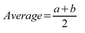
Yes they are. What is a ‘weighted’ average? Well, lets take our bog-standard average of two numbers a and b

For any average, the numerator on top is the sum of the numbers, and the denominator below is how many numbers we are averaging. I am only interested in when we have two numbers. Programmers will be more familiar with multiplying by 0.5:

Well, if we say that α = 0.5, knowing that 0.5 = 1-0.5, then we can write the equation in this form:

So there you have it, provided that the sum of (1-γ) and γ is equal to 1.0, we can write any averaging equation in this form.

It is a weighted average when (1-γ) does not equal γ (and does not equal 0.5), in which case the term with the largest coefficient will have more impact on our result. In other words the value of A will be influenced by the proportions of a and b coming through. For example, If γ = 0.9, then A is equal to 10% of a and 90% of b.

Equation 1.3 is often used to describe transparency, or alpha blending, as it is in Jason Gregory’s book Game Engine Architecture. This is because if we have two pixels, and one is supposed to be semi-transparent, then we calculate this transparency by calculating the proportion of each pixel on the final colour.

Personally, however, if a and b were coordinates, which we will now call Pa and Pb, then for moving an object between two points I don’t find the above form very intuitive. Lets rearrange:

There we go. This is intuitive. If γ is zero, the P’ = Pa. If however γ is 1, then we have P’ = Pa + Pb – Pa = Pa-Pa + Pb = Pb. It is now about the sliding scale from γ = 0 to γ = 1, which is exactly what we want. A sliding scale from two numbers, points, vectors, whatever: source to destination.

Thanks James! Hangon.. How do I use this?

γ is a float within the range 0.0<=γ<=1.0. So if we are interpolating something over time, then you can calculate the progress of your timer. In other words, use the proportion of how long into your total duration you are currently. A game timer class can do this, for example I have some older C# code below:

As you can see, this is the same equation as above.

Linear vs non-linear?

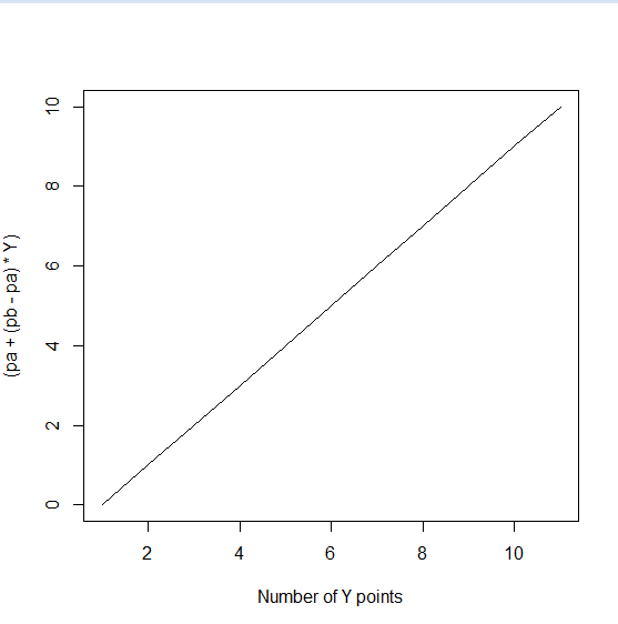
If γ grows by a constant value at each interval, then it will be growing linearly. Hence the term Linear-intERPolation, often shortened to just “Lerp”. If we were to plot P’ as above when interpolting linearly between Pa and Pb, then we would have a straight diaganol line over all values of γ (0 to 1) from Pa to Pb.

To achieve a non-linear interpolation, we instead need a “smooth function” of γ.

Non-linear interpolations

Binomial

A simple equation to achieve a smooth function of γ, or h, or t, or whatever you want to call the proportion in which we interpolate by, is given below:

As stated in the caption, this assumes x is between 0 and 1 (and when you are programming this, it will only work with a float or double). The function is what is called monomolecular:

Why does this work? Because x squared, if x is between 0 and 1 will converge to 1, but never quite get there. As 1* 1 = 1, the closer x is to 1, the smaller the effect of squaring it. Having the first term be equal to 2, means that γ will be between 0 and 1, which is what we want.

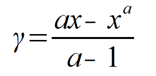
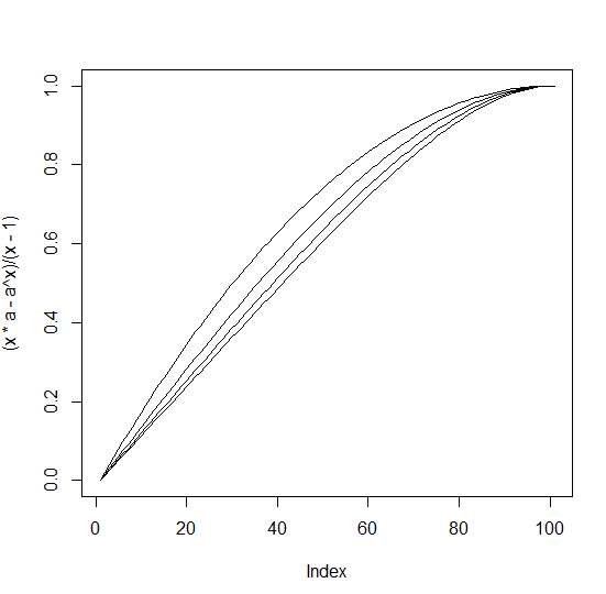
We can change the rate of growth of this function. The above listing is incomplete. The coefficient and power, can be any other value except for 2. We will call this value a. But to allow for proportionality between growth of the two terms, we need to normalise the function, by dividing by a-1:

At greater values of a, the rate of growth is increased, and our curvature decreases. You can also reduce a, provided that it is greater than 1, to avoid a divide by zero error.

To be continued!